Zero-Shot Machine Learning in SQL: Predictions Without a Training Loop

You have 120 labelled rows and 30 unlabelled ones. The classical answer is a Python project. The new answer is one SELECT.

SELECT * FROM tabfm_classify('iris', 'species');

No training loop. No feature engineering. No model artifact to version. The model reads your labelled rows as context and predicts the rest—the same way an LLM learns from examples in a prompt.

Every number and every terminal recording in this post was produced on an 8-core CPU against public Hugging Face datasets. Nothing is simulated.

The Problem: Most Predictions Aren't Worth a Model

Here is a task that lands on a data team's desk every week:

"We have 4,000 parts. 3,100 have a material group. 900 are blank. Can you fill them in?"

Technically, this is supervised classification. Practically, nobody wants to build it. The honest cost estimate looks like this:

• -> Export the data. Out of the warehouse, into a notebook. Now you have two copies of the truth.
• -> Build a feature pipeline. Encode the categoricals, impute the nulls, scale the numerics. Then rebuild it identically for inference, or your predictions silently drift.
• -> Pick and tune a model. Gradient boosting, probably. Cross-validate. Tune. Justify.
• -> Ship it. Somewhere to store the artifact. Something to retrain it. Someone to own it.

Two weeks of work for a column. So the column stays blank, or someone fills it in by hand, or a junior analyst writes 40 CASE WHEN branches that nobody dares touch again.

The economics are backwards: the machinery costs more than the problem.

What Changed: The Model Comes Pre-Trained on Tables

Large language models broke this pattern for text. You don't fine-tune a model to classify a support ticket—you put five examples in the prompt and it works. That's in-context learning: the model was pre-trained so broadly that your specific task becomes an input, not a training job.

Tabular foundation models do the same thing for rows and columns. The pioneering work here is TabPFN (Prior Labs, published in Nature in 2025): a transformer pre-trained on millions of synthetic tabular datasets until it learned, in general, how tables behave. At inference it takes your labelled rows as context and your unlabelled rows as queries, and does one forward pass.

The consequences are what make this interesting:

Classical ML	Tabular foundation model
Fit on your data, then predict	One forward pass, nothing fitted
Model artifact per task	One model, every task
Needs enough rows to learn	Works well from ~100 rows
Feature encoding is your job	Handles mixed types natively
Retrain when data shifts	Add rows to the context

There is no artifact because there is no training. Change your data, and the next query already reflects it.

And—this is the part that matters for a database—the whole thing is one forward pass over a table. That is exactly the shape of a SQL operator.

The Extension: anofox_tabfm

anofox_tabfm embeds ONNX Runtime in DuckDB and exposes tabular foundation models as table functions. Install it from the community repository:

INSTALL anofox_tabfm FROM community;
LOAD anofox_tabfm;

INSTALL httpfs;   -- model weights are fetched over HTTPS
LOAD httpfs;

The extension ships weight-free graphs. The weights are your own Hugging Face download, once, cached under ~/.cache/anofox-tabfm:

CALL tabfm_download('classification', model := 'mitra');   -- 303 MB, Apache-2.0

mitra is a good default: AWS's tabular foundation model, Apache-2.0 licensed, small, no license gate. Three more models ship built in—more on that below.

Sixty Seconds With Real Data

Let's use the iris dataset, because you can hold all of it in your head: four flower measurements, three species. We read it straight from Hugging Face and hide 20% of the labels so we have something to predict.

CREATE TABLE iris AS
SELECT round(SepalLengthCm, 1) AS sepal_len,
       round(SepalWidthCm, 1)  AS sepal_wid,
       round(PetalLengthCm, 1) AS petal_len,
       round(PetalWidthCm, 1)  AS petal_wid,
       CASE WHEN row_number() OVER () % 5 = 0
            THEN NULL ELSE replace(Species, 'Iris-', '') END AS species
FROM 'hf://datasets/scikit-learn/iris/**/*.csv';

150 rows: 120 with a species, 30 without. The 120 labelled rows are the context. The 30 NULL rows are what we want. That is the entire configuration—here it is running for real:

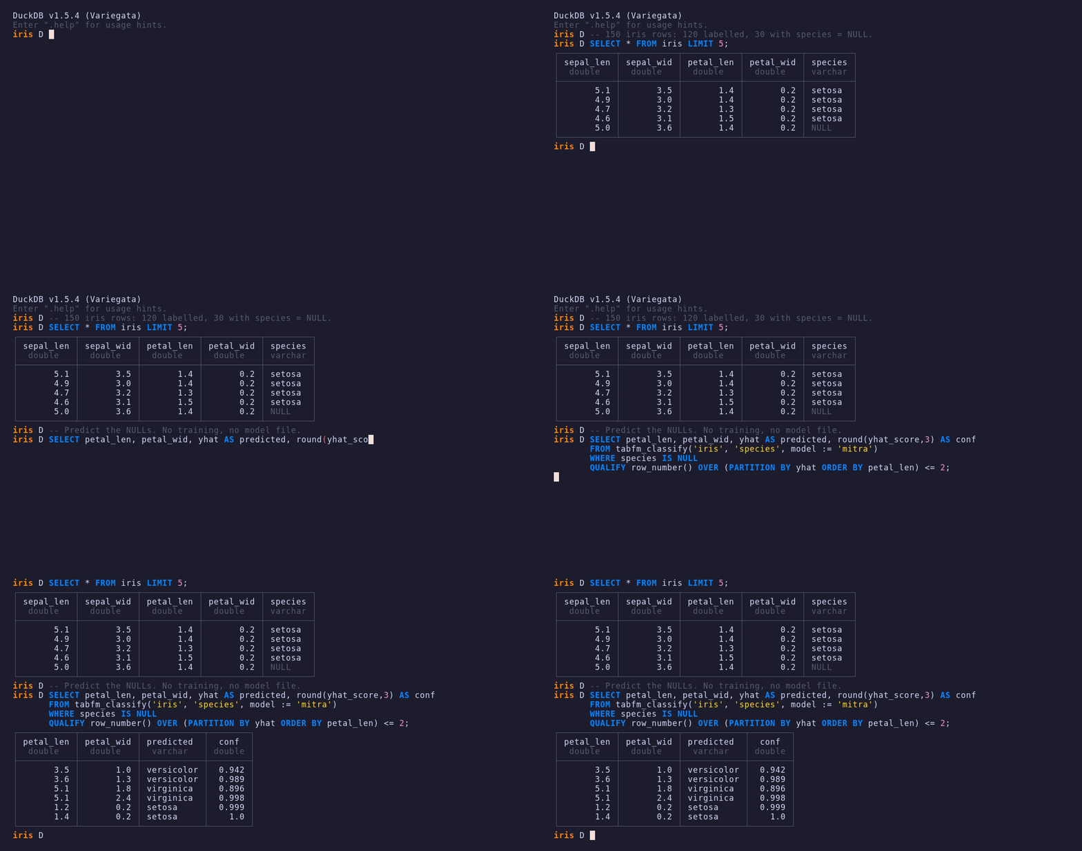
The query, in full:

SELECT petal_len, petal_wid, yhat AS predicted, round(yhat_score, 3) AS conf
FROM tabfm_classify('iris', 'species', model := 'mitra')
WHERE species IS NULL
QUALIFY row_number() OVER (PARTITION BY yhat ORDER BY petal_len) <= 2;

petal_len	petal_wid	predicted	conf
3.5	1.0	versicolor	0.942
3.6	1.3	versicolor	0.989
5.1	1.8	virginica	0.896
5.1	2.4	virginica	0.998
1.2	0.2	setosa	0.999
1.4	0.2	setosa	1.000

Two seconds, a foundation model, nothing installed but a DuckDB extension. Held out properly—97 context rows, 53 rows scored blind—mitra gets 96.2% of them right.

The two shapes

Both functions share one signature; the task is fixed by which one you call.

tabfm_classify(data, target [, test] [, features] [, opts])
tabfm_regress (data, target [, test] [, features] [, opts])

Single relation (what we just did): rows whose target IS NULL are the ones to score. Every row comes back with an is_training flag, so you can sanity-check the fitted values on rows you already know.

Explicit train/test—the familiar fit(X_train, y_train).predict(X_test) shape. Only the scored rows come back:

SELECT * FROM tabfm_classify('history', 'churned', test := 'prospects');

A subquery works anywhere a table name does:

SELECT * FROM tabfm_classify(
    '(SELECT * FROM history WHERE signup_year = 2025)', 'churned',
    test := 'prospects');

You get these columns back alongside every column of the scored rows:

column	meaning
yhat	predicted label (classification) or value (regression)
yhat_score	probability of the top class; NULL for regression
proba	MAP(label → probability)—the full distribution
is_training	single-relation mode: was this a context row?

Does It Work on Real Business Data?

Iris is a demo. Let's try something with the texture of an actual operational table: telco customer churn—7,043 customers, 20 mixed-type columns, an imbalanced target.

CREATE TABLE churn AS
SELECT *, hash(customerID) % 100 AS bucket
FROM 'hf://datasets/scikit-learn/churn-prediction/**/*.csv';

customerID	gender	tenure	Contract	MonthlyCharges	TotalCharges	Churn
7590-VHVEG	Female	1	Month-to-month	29.85	29.85	false
5575-GNVDE	Male	34	One year	56.95	1889.5	false
3668-QPYBK	Male	2	Month-to-month	53.85	108.15	true
7795-CFOCW	Male	45	One year	42.30	1840.75	false
9237-HQITU	Female	2	Month-to-month	70.70	151.65	true

Booleans, categoricals with six levels, a numeric column that arrived as text, and 1,869 churners against 5,174 non-churners. No encoding, no imputation, no scaling—hand it over as-is.

A deterministic split by hash, so this is reproducible:

CREATE TABLE train AS SELECT * EXCLUDE (bucket)
  FROM (FROM churn WHERE bucket < 70) USING SAMPLE 500 ROWS (reservoir, 42);
CREATE TABLE test AS SELECT * EXCLUDE (bucket)
  FROM (FROM churn WHERE bucket >= 70) USING SAMPLE 300 ROWS (reservoir, 42);
CREATE TABLE test_features AS SELECT * EXCLUDE (Churn) FROM test;   -- labels withheld

Predict:

CREATE TABLE preds AS
SELECT customerID, yhat AS pred, yhat_score
FROM tabfm_classify('train', 'Churn', test := 'test_features', model := 'mitra');

customerID	pred	yhat_score
2351-BKRZW	false	0.985
4373-MAVJG	true	0.586
2921-XWDJH	false	0.592
4139-SUGLD	false	0.811
4729-XKASR	true	0.653

Then score it against the held-out labels—also in SQL:

WITH cm AS (
  SELECT count(*) FILTER (WHERE p.pred AND t.Churn)         AS tp,
         count(*) FILTER (WHERE p.pred AND NOT t.Churn)     AS fp,
         count(*) FILTER (WHERE NOT p.pred AND t.Churn)     AS fn,
         count(*) FILTER (WHERE NOT p.pred AND NOT t.Churn) AS tn
  FROM preds p JOIN test t USING (customerID))
SELECT tp, fp, fn, tn,
       round((tp + tn)::DOUBLE / (tp + fp + fn + tn), 3)    AS accuracy,
       round(tp::DOUBLE / nullif(tp + fp, 0), 3)            AS precision,
       round(tp::DOUBLE / nullif(tp + fn, 0), 3)            AS recall,
       round(2.0 * tp / nullif(2.0 * tp + fp + fn, 0), 3)   AS f1
FROM cm;

tp	fp	fn	tn	accuracy	precision	recall	f1
50	15	53	182	0.773	0.769	0.485	0.595

Read that honestly. Precision 0.77 on 500 context rows and zero training: when the model flags a customer as churning, it is right roughly three times out of four. Recall 0.485 is the weak half—it misses about half the churners. That is a threshold you can move (proba gives you the full distribution), not a broken model.

Compare it to the alternatives you actually have on a Tuesday afternoon: a two-week ML project, or nothing. This was one query and 23 seconds.

The surprise: you don't need all your data

The obvious next move is "throw more rows at it." We ran the same held-out 300 customers against three context sizes:

context rows	accuracy	precision	recall	F1	time
100	0.740	0.687	0.447	0.541	8 s
500	0.773	0.769	0.485	0.595	23 s
2,000	0.767	0.780	0.447	0.568	78 s

Going from 100 to 500 context rows bought a real improvement. Going from 500 to 2,000 bought nothing—and cost 3.4× the time. Inference scales with context, so the last quadrupling was pure expense.

This inverts a habit. With classical ML, more labelled data is almost always better and it is free at inference time. With in-context learning, the context is the inference cost. A few hundred well-chosen rows is often the whole game—which is also why this works at all on the tables where you only have a few hundred labelled rows.

Four Models, One Keyword

"TabFM" is a category, not a product. The field moved fast, and four models ship built into the extension—usable by name, with no manifest file and no configuration:

SELECT model, license, commercial FROM tabfm_list_models();

model	family	license	commercial
mitra	AWS AutoGluon	apache-2.0	true
tabpfn-v2	Prior Labs	apache-2.0	true
tabicl-v2	Inria	bsd-3-clause	true
tabfm-v1	Google TabFM	tabfm-non-commercial-v1.0	false

Switching models is a keyword:

SELECT * FROM tabfm_classify('iris', 'species', model := 'tabicl-v2');
SET anofox_tabfm_default_model = 'mitra';   -- or set it once per session

Which means comparing them is a query, not a research project. Same context, same held-out rows, one word changed:

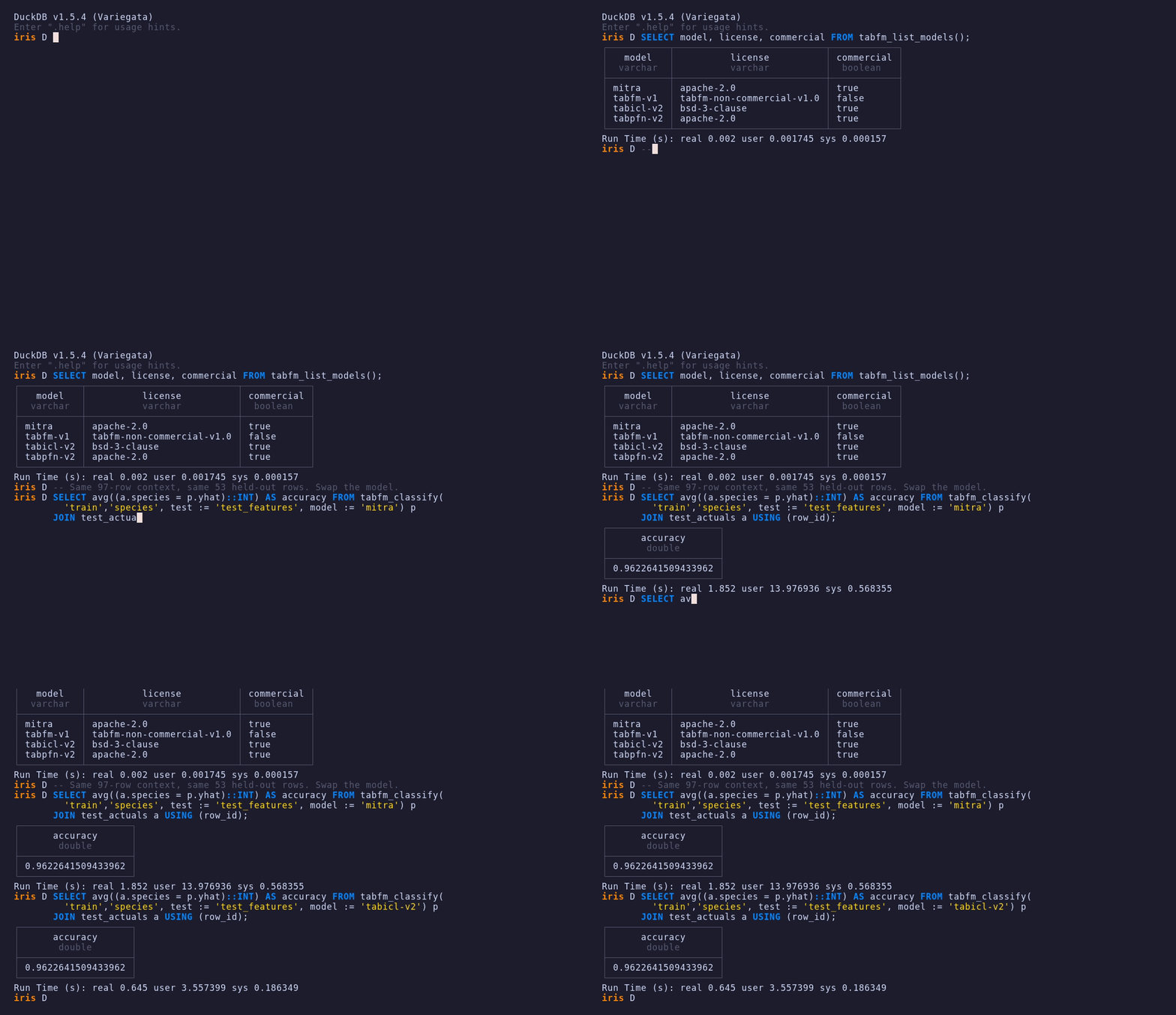
Run across three of the built-in models on the same 97-row context and 53 held-out iris rows:

model	size	license	accuracy	runtime
tabicl-v2	110 MB	BSD-3-Clause	0.962	0.54 s
mitra	303 MB	Apache-2.0	0.962	1.57 s
tabfm-v1	6.56 GB	non-commercial	0.943	28.25 s

The 110 MB BSD-licensed model is more accurate than the 6.56 GB gated one, and 52× faster. Bigger is emphatically not better here, and the permissive licences are on the models you would actually want to use. Being able to establish that with one changed word—rather than four separate integrations—is the point of the registry.

You can also register your own model entirely in SQL: CALL tabfm_register_model(id := 'my', classification_graph := '<path|url>', …). The only external artifact is a weight-free ONNX graph; every other field is a named argument. Adding a model is a data change, not a code change.

(One caveat we hit while writing this: tabpfn-v2's published checkpoint did not load against the bundled graph in the current release, so it is absent from the table above rather than reported second-hand. The other three ran clean.)

Regression, Same Shape

tabfm_regress takes identical arguments and predicts numbers instead of labels. Restaurant tips—186 context rows, 58 held out, predicting the tip from the bill, party size, day, and time:

CREATE TABLE preds AS
SELECT row_id, yhat AS pred
FROM tabfm_regress('train', 'tip', test := 'test_features', model := 'tabfm-v1');

total_bill	size	predicted_tip	actual_tip
20.29	2	3.19	2.75
19.82	2	3.12	3.18
12.69	2	2.09	2.00
19.65	2	3.13	3.00
9.55	2	1.70	1.45
18.35	4	2.72	2.50

model	MSE	RMSE	MAE	vs. mean baseline
tabfm-v1	0.986	0.993	0.713	22% better
mitra	1.187	1.089	0.912	7% better
predict the mean	1.271	—	—	—

Regression is the weaker half of the story, and the model ranking flips: here the big Google model clearly beats Mitra, the reverse of the classification result. If regression is your workload, benchmark on your data before picking—which, again, is one keyword.

The Honest Limits

Zero-shot in-context learning has real trade-offs. Know them before you build on it:

• -> Context has a ceiling. The guardrail is anofox_tabfm_max_rows (default 10,000) per predict, and each model has its own supported maximum—tabicl-v2 goes to 100,000, mitra and tabpfn-v2 to 10,000. This is a tool for operational tables, not for a billion-row fact table.
• -> Feature width matters. 100 features for mitra, 500 for tabpfn-v2, 512 for tabicl-v2. Classification tops out at 10 classes on the permissive models.
• -> Inference is compute, not lookup. Scoring 300 churn rows against 500 context rows took 23 seconds on 8 CPU cores; the same job with 2,000 context rows took 78. There are cuda, rocm, and coreml builds when that matters.
• -> Weights are your download, under their licence. The extension is MIT and ships zero weight bytes. mitra, tabpfn-v2, and tabicl-v2 are commercially usable; Google's tabfm-v1 is gated and non-commercial, and refuses to download until you SET anofox_tabfm_accept_hf_license = true.
• -> A tuned model on lots of data still wins. With 500,000 labelled rows and a stable target, train the gradient-boosted tree. Foundation models shine exactly where classical ML is uneconomical: few rows, many small tasks, changing data.

Everything that can fail raises a DuckDB exception that names the fix:

Invalid Input Error: tabfm: model 'classification' is not downloaded.
Run: CALL tabfm_download('classification');

Try It on Your Own Table

Find a column in your warehouse that is mostly filled in and partly blank. That is the whole prerequisite.

INSTALL anofox_tabfm FROM community;
LOAD anofox_tabfm;
INSTALL httpfs; LOAD httpfs;

CALL tabfm_download('classification', model := 'mitra');   -- once, 303 MB

SELECT * FROM tabfm_classify('your_table', 'the_mostly_filled_column')
WHERE the_mostly_filled_column IS NULL;

Start with something you can verify: hide labels you already have, predict them back, count how many the model gets right. Two hundred context rows is enough for a first read.

If it works on your data the way it worked on ours, the next question is not "should we build a model?"—it is "which columns should we stop filling in by hand?"

---

In this series:

1. Zero-Shot Machine Learning in SQL — in-context learning, the two shapes, measured results (this post)
2. Which Tabular Foundation Model Should You Use? — three models, five datasets, measured
3. Foundation Models in Production — cost, memory, and air-gapped deployment

---

Reference

📖 anofox-tabfm on GitHub → — full SQL API, runnable examples, and the benchmark scripts behind every number in this post.